interest rate, Meta Intelligence

Economics-Watching: “Doing Nothing” Is Still Doing a Lot

[from the Federal Reserve Bank of Philadelphia, speech by Patrick T. Harker President and Chief Executive Officer at the National Association of Corporate Directors Webinar, Philadelphia, PA (Virtual)]

Good afternoon, everyone.

I appreciate that you’re all giving up part of the end of your workday for us to be together, if only virtually.

My thanks to my good friend, Rick Mroz, for that welcome and introduction.

I do believe we’re going to have a productive session. But just so you all know, as much as I enjoy speaking and providing my outlook, I enjoy a good conversation even more.

So, first, let’s take a few minutes so I can give you my perspective on where we are headed, and then I will be more than happy to take questions and hear what’s on your minds.

But before we get into any of that, I must begin with the standard Fed disclaimer: The views I express today are my own and do not necessarily reflect those of anyone else on the Federal Open Market Committee (FOMC) or in the Federal Reserve System.

Put simply, this is one of those times where the operative words are, “Pat said,” not “the Fed said.”

Now, to begin, I’m going to first address the two topics that I get asked about most often: interest rates and inflation. And I would guess they are the topics front and center in many of your minds as well.

After the FOMC’s last policy rate hike in July, I went on record with my view that, if economic and financial conditions evolved roughly as I expected they would, we could hold rates where they are. And I am pleased that, so far, economic and financial conditions are evolving as I expected, if not perhaps even a tad better.

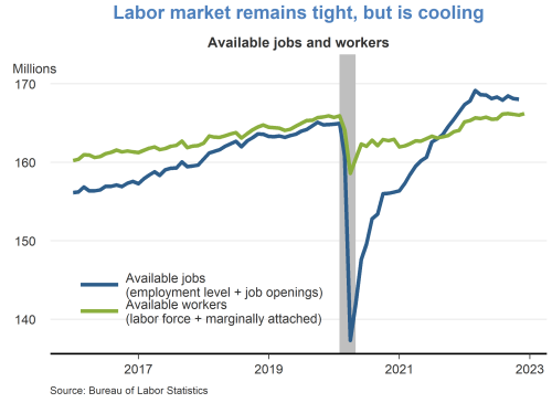
Let’s look at the current dynamics. There is a steady, if slow, disinflation under way. Labor markets are coming into better balance. And, all the while, economic activity has remained resilient.

Given this, I remain today where I found myself after July’s meeting: Absent a stark turnabout in the data and in what I hear from contacts, I believe that we are at the point where we can hold rates where they are.

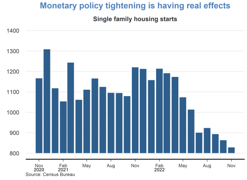
In barely more than a year, we increased the policy rate by more than 5 percentage points and to its highest level in more than two decades — 11 rate hikes in a span of 12 meetings prior to September. We not only did a lot, but we did it very fast.

We also turned around our balance sheet policy — and we will continue to tighten financial conditions by shrinking the balance sheet.

The workings of the economy cannot be rushed, and it will take some time for the full impact of the higher rates to be felt. In fact, I have heard a plea from countless contacts, asking to give them some time to absorb the work we have already done.

I agree with them. I am sure policy rates are restrictive, and, as long they remain so, we will steadily press down on inflation and bring markets into a better balance.

Holding rates steady will let monetary policy do its work. By doing nothing, we are still doing something. And I would argue we are doing quite a lot.

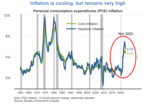
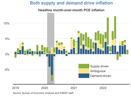
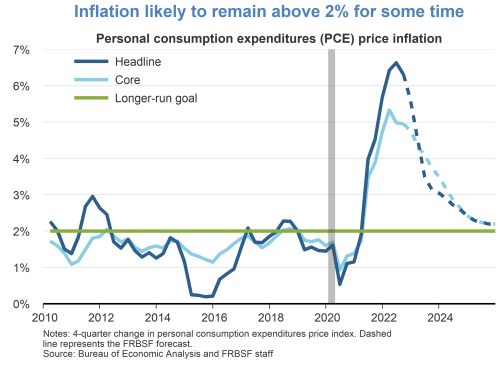
Headline PCE inflation remained elevated in August at 3.5 percent year over year, but it is down 3 percentage points from this time last year. About half of that drop is due to the volatile components of energy and food that, while basic necessities, they are typically excluded by economists in the so-called core inflation rate to give a more accurate assessment of the pace of disinflation and its likely path forward.

Well, core PCE inflation has also shown clear signs of progress, and the August monthly reading was its smallest month-over-month increase since 2020.

So, yes, a steady disinflation is under way, and I expect it to continue. My projection is that inflation will drop below 3 percent in 2024 and level out at our 2 percent target thereafter.

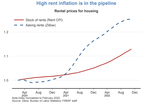
However, there can be challenges in assessing the trends in disinflation. For example, September’s CPI report came out modestly on the upside, driven by energy and housing.

Let me be clear about two things. First, we will not tolerate a reacceleration in prices. But second, I do not want to overreact to the normal month-to-month variability of prices. And for all the fancy techniques, the best way to separate a signal from noise remains to average data over several months. Of course, to do so, you need several months of data to start with, which, in turn, demands that, yes, we remain data-dependent but patient and cautious with the data.

Turning to the jobs picture, I do anticipate national unemployment to end the year at about 4 percent — just slightly above where we are now — and to increase slowly over the next year to peak at around 4.5 percent before heading back toward 4 percent in 2025. That is a rate in line with what economists call the natural rate of unemployment, or the theoretical level in which labor market conditions support stable inflation at 2 percent.

Now, that said, as you know, there are many factors that play into the calculation of the unemployment rate. For instance, we’ve seen recent months where, even as the economy added more jobs, the unemployment rate increased because more workers moved off the sidelines and back into the labor force. There are many other dynamics at play, too, such as technological changes or public policy issues, like child care or immigration, which directly impact employment.

And beyond the hard data, I also have to balance the soft data. For example, in my discussions with employers throughout the Third District, I hear that given how hard they’ve worked to find the workers they currently have, they are doing all they can to hold onto them.

So, to sum up the labor picture, let me say, simply, I do not expect mass layoffs.

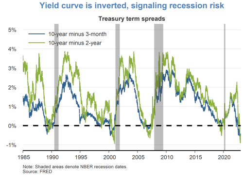
I do expect GDP gains to continue through the end of 2023, before pulling back slightly in 2024. But even as I foresee the rate of GDP growth moderating, I do not see it contracting. And, again, to put it simply, I do not anticipate a recession.

Look, this economy has been nothing if not unpredictable. It has proven itself unwilling to stick to traditional modeling and seems determined to not only bend some rules in one place, but to make up its own in another. However, as frustratingly unpredictable as it has been, it continues to move along.

And this has led me to the following thought: What has fundamentally changed in the economy from, say, 2018 or 2019? In 2018, inflation averaged 2 percent almost to the decimal point and was actually below target in 2019. Unemployment averaged below 4 percent for both years and was as low as 3.5 percent — both nationwide and in our respective states — while policy rates peaked below 2.5 percent.

Now, I’m not saying we’re going to be able to exactly replicate the prepandemic economy, but it is hard to find fundamental differences. Surely, I cannot and will not minimize the immense impacts of the pandemic on our lives and our families, nor the fact that for so many, the new normal still does not feel normal. From the cold lens of economics, I do not see underlying fundamental changes. I could also be wrong, and, trust me, that would not be the first time this economy has made me rethink some of the classic models. We just won’t know for sure until we have more data to look at over time.

And then, of course, there are the economic uncertainties — both national and global — against which we also must contend. The ongoing auto worker strike, among other labor actions. The restart of student loan payments. The potential of a government shutdown. Fast-changing events in response to the tragic attacks against Israel. Russia’s ongoing war against Ukraine. Each and every one deserves a close watch.

These are the broad economic signals we are picking up at the Philadelphia Fed, but I would note that the regional ones we follow are also pointing us forward.

First, while in the Philadelphia Fed’s most recent business outlook surveys, which survey manufacturing and nonmanufacturing firms in the Third District, month-over-month activity declined, the six-month outlooks for each remain optimistic for growth.

And we also publish a monthly summary metric of economic activity, the State Coincident Indexes. In New Jersey, the index is up slightly year over year through August, which shows generally positive conditions. However, the three-month number from June through August was down, and while both payroll employment and average hours worked in manufacturing increased during that time, so did the unemployment rate — though a good part of that increase can be explained as more residents moved back into the labor force.

And for those of you joining us from the western side of the Delaware River, Pennsylvania’s coincident index is up more than 4 percent year over year through August and 1.7 percent since June. Payroll employment was up, and the unemployment rate was down; however, the number of average hours worked in manufacturing decreased.

There are also promising signs in both states in terms of business formation. The number of applications, specifically, for high-propensity businesses — those expected to turn into firms with payroll — are remaining elevated compared with pre-pandemic levels. Again, a promising sign.

So, it is against this full backdrop that I have concluded that now is the time at which the policy rate can remain steady. But I can hear you ask: “How long will rates need to stay high.” Well, I simply cannot say at this moment. My forecasts are based on what we know as of late 2023. As time goes by, as adjustments are completed, and as we have more data and insights on the underlying trends, I may need to adjust my forecasts, and with them my time frames.

I can tell you three things about my views on future policy. First, I expect rates will need to stay high for a while.

Second, the data and what I hear from contacts and outreach will signal to me when the time comes to adjust policy either way. I really do not expect it, but if inflation were to rebound, I know I would not hesitate to support further rate increases as our objective to return inflation to target is, simply, not negotiable.

Third, I believe that a resolute, but patient, monetary policy stance will allow us to achieve the soft landing that we all wish for our economy.

Before I conclude and turn things over to Rick to kick off our Q&A, I do want to spend a moment on a topic that he and I recently discussed, and it’s something about which I know there is generally great interest: fintech. In fact, I understand there is discussion about NACD hosting a conference on fintech.

Well, last month, we at the Philadelphia Fed hosted our Seventh Annual Fintech Conference, which brought business and thought leaders together at the Bank for two days of real in-depth discussions. And I am extraordinarily proud of the fact that the Philadelphia Fed’s conference has emerged as one of the premier conferences on fintech, anywhere. Not that it’s a competition.

I had the pleasure of opening this year’s conference, which always puts a focus on shifts in the fintech landscape. Much of this year’s conference centered around developments in digital currencies and crypto — and, believe me, some of the discussions were a little, shall we say, “spirited.” However, my overarching point to attendees was the following: Regardless of one’s views, whether in favor of or against such currencies, our reality requires us to move from thinking in terms of “what if” to thinking about “what next.”

In many ways, we’re beyond the stage of thinking about crypto and digital currency and into the stage of having them as reality — just as AI has moved from being the stuff of science fiction to the stuff of everyday life. What is needed now is critical thinking about what is next. And we at the Federal Reserve, both here in Philadelphia and System-wide, are focused on being part of this discussion.

We are also focused on providing not just thought leadership but actionable leadership. For example, the Fed rolled out our new FedNow instant payment service platform in July. With FedNow, we will have a more nimble and responsive banking system.

To be sure, FedNow is not the first instant payment system — other systems, whether operated by individual banks or through third parties, have been operational for some time. But by allowing banks to interact with each other quickly and efficiently to ensure one customer’s payment becomes another’s deposit, we are fulfilling our role in providing a fair and equitable payment system.

Another area where the Fed is assuming a mantle of leadership is in quantum computing, or QC, which has the potential to revolutionize security and problem-solving methodologies throughout the banking and financial services industry. But that upside also comes with a real downside risk, should other not-so-friendly actors co-opt QC for their own purposes.

Right now, individual institutions and other central banks globally are expanding their own research in QC. But just as these institutions look to the Fed for economic leadership, so, too, are they looking to us for technological leadership. So, I am especially proud that this System-wide effort is being led from right here at the Philadelphia Fed.

I could go on and talk about fintech for much longer. After all, I’m actually an engineer more than I am an economist. But I know that Rick is interested in starting our conversation, and I am sure that many of you are ready to participate.

But one last thought on fintech — my answers today aren’t going to be generated by ChatGPT.

On that note, Rick, thanks for allowing me the time to set up our discussion, and let’s start with the Q&A.

[archived PDF of the above speech]

FRBSF Economic Letter: Can Monetary Policy Tame Rent Inflation?

[from the Federal Reserve Bank of San Francisco Economic Letter]

by Zheng Liu and Mollie Pepper

Rent inflation has surged since early 2021. Because the cost of housing is an important component of total U.S. consumer spending, high rent inflation has contributed to elevated levels of overall inflation. Evidence suggests that, as monetary policy tightening cools housing markets, it can also reduce rent inflation, although this tends to adjust relatively slowly. A policy tightening equivalent to a 1 percentage point increase in the federal funds rate could reduce rent inflation as much as 3.2 percentage points over 2½ years.

“We’ve had a time of red-hot housing market all over the country… Shelter inflation is going to remain high for some time. We’re looking for it to come down, but it’s not exactly clear when that will happen. Hope for the best, plan for the worst.”
Federal Reserve Chair Jerome Powell (2022)

The rapid run-up of shelter costs—both house prices and rents—during the recovery from the pandemic has raised questions about how inflation pressures might affect housing affordability. Since March 2022, the Federal Reserve has rapidly lifted its federal funds rate target from near zero to over 4%, and policymakers have signaled that they are open to keeping the monetary policy stance sufficiently restrictive to return inflation to the longer-run goal of 2% on average. The tightened financial conditions following those policy changes, especially the surge in mortgage interest rates, have helped cool house price growth. However, rent inflation remains elevated.

This Economic Letter examines the effectiveness of monetary policy tightening for reducing rent inflation. We estimate that, during the period from 1988 to 2019, a policy tightening equivalent to a 1 percentage point increase in the federal funds rate can reduce rent inflation—measured by 12-month percentage changes in the personal consumption expenditures (PCE) housing price index—by about 3.2 percentage points, but the full impact takes about 2½ years to materialize. Based on housing costs’ share in total PCE, this translates to a reduction in headline PCE inflation of about 0.5 percentage point over the same time horizon.

Rising housing costs

Following the COVID-19 recession, house prices and rents both surged in the United States. For example, the 12-month growth rate of Standard & Poor’s CoreLogic Case-Shiller Home Price Index accelerated from about 10% in December 2020 to over 20% in March 2022. After the Federal Reserve started raising the target for the federal funds rate in March, house price growth has slowed significantly, to about 9% in October 2022.

Rent inflation also accelerated during the pandemic period. Figure 1 shows that rent inflation—measured using 12-month changes in the PCE housing price index and including rents for tenant-occupied housing and imputed rents for owner-occupied housing—rose from a low point of about 2% in early 2021 to 7.7% by December 2022, the highest level since 1986. During the same period, rent inflation measured by 12-month changes in the shelter component of the consumer price index (CPI) experienced a similar increase. Thus, following the tightening of monetary policy, house price growth has slowed but rent inflation continues to rise.

Figure 1: PCE and CPI measures of rent inflation

Source: Bureau of Economic Analysis, Bureau of Labor Statistics, and Haver Analytics.
Note: Twelve-month percentage changes. Gray shading indicates NBER recession dates.

Economic theory suggests that some common forces such as changes in housing demand can drive both rents and house prices. For example, the expansion of remote work since the COVID-19 pandemic has increased demand for housing, raising both house prices and rents (Kmetz, Mondragon, and Wieland 2022). To the extent that the stream of current and future rents reflects the fundamental value of a house, house prices can be a leading indicator of future rent inflation (Lansing, Oliveira, and Shapiro 2022). Thus, monetary policy can affect both house prices and rents by cooling housing demand.

Housing demand responds to changes in financial conditions, such as increases in mortgage interest rates. However, theory suggests that house prices are more sensitive than rental prices to changes in financial conditions, because home purchases typically require longer-term mortgage financing. In addition, unlike rents, house prices can be partly driven by investor sentiments or beliefs, which explains the observed larger swings in house prices than in rents over business cycles (Dong et al. 2022). Long-term rental contracts can also contribute to slow adjustments in rent inflation.

Rent inflation is an important contributor to overall inflation because housing costs are an important component of total consumption expenditures. On average, housing expenditures represent about 15% of total PCE and 25% of the services component of PCE. In CPI, shelter costs represent an even larger share, accounting for about 30% of total consumption of all urban consumers and about 40% of core consumption expenditures excluding volatile food and energy components.

The contribution of rent inflation to overall PCE inflation has increased since early 2021. As Figure 2 shows, in the first quarter of 2021, rent inflation accounted for about 22% of the four-quarter change in the PCE services price index, excluding energy: 0.5 of the 2.3 percentage points increase in service prices was attributable to rent inflation. By the third quarter of 2022, the contribution of rent inflation had climbed to about one-third, or 1.5 of the 4.7 percentage point increase in service prices.

Figure 2: Rising contribution of rent inflation to services inflation

Source: Bureau of Economic Analysis, Haver Analytics, and authors’ calculations.
Note: Four-quarter changes in PCE services price index excluding energy.

Measuring policy effects

Given the rising contribution of rent inflation to overall inflation, it is important to assess the quantitative effects of monetary policy tightening on rent inflation.

For our analysis, we use a measure of monetary policy surprises constructed by Bauer and Swanson (2022). Their measure focuses on high-frequency changes in financial market indicators within a short period surrounding the Federal Open Market Committee (FOMC) policy announcements. If the public fully anticipates a policy change, then the financial market would not react to new policy announcements. However, if the market does react to an announcement, then the policy change must contain a surprise element. Thus, changes in financial market indicators, such as the price of Eurodollar futures, in a narrow window around an FOMC announcement can capture policy surprises. In practice, however, the data constructed this way are not complete surprises because they can be predicted by some macro and financial variables shortly before FOMC announcements. We follow the approach of Bauer and Swanson (2022) to purge the influences of those macro and financial variables from the measure of policy surprises. We use the resulting quarterly time series to measure monetary policy shocks, with a sample period from 1988 to 2019.

We then use a local projections model—a statistical tool proposed by Jordà (2005)—to project how rent inflation responds over time to a tightening of monetary policy equivalent to a 1 percentage point unanticipated increase in the federal funds rate in a given quarter. The model takes into account how monetary policy shocks interact with other macroeconomic variables, including lags of rent inflation, real GDP growth, and core PCE inflation.

In the final step, we compute the responses of rent inflation relative to its preshock level over a period up to 20 quarters after the initial increase in the federal funds rate.

Gradual impact of policy tightening on rent inflation

Figure 3 shows the response of rent inflation during the first 20 quarters after an unanticipated tightening of monetary policy (solid blue line). The shaded area shows the confidence band, indicating the statistical uncertainty in estimating the responses. Under the assumption that the model is correct, the shaded area contains the actual value of the rent inflation responses to the monetary policy shock roughly two-thirds of the time. The policy shock is normalized such that it is equivalent to a 1 percentage point unanticipated increase in the federal funds rate.

Figure 3: Response of rent inflation to monetary policy tightening

Source: Bureau of Economic Analysis, Bauer and Swanson (2022), and authors’ calculations.
Note: Response of rent inflation to a monetary policy shock equivalent to a 1 percentage point surprise increase in the federal funds rate. Shaded region shows 68% confidence band around the estimate.

The figure shows that monetary policy tightening has significant and gradual effects on rent inflation. On impact, a 1 percentage point increase in the federal funds rate reduces rent inflation about 0.6 percentage point relative to its preshock level. Over time, rent inflation declines gradually, falling about 3.2 percentage points in the 10 quarters following the impact. The slow adjustment in rent inflation partly reflects the stickiness in nominal rents due to long-term rental contracts. Since housing expenditures account for about 15% of total PCE, this estimate translates to a reduction in headline PCE inflation of about 0.5 percentage point, stemming from the decline in rent inflation over a period of 2½ years.

The rent component of PCE is measured based on average rents, including those locked in long-term rental contracts, which are slow to adjust to changes in economic and financial conditions. Rents on new leases, however, are more flexible. For example, the 12-month growth in Zillow’s observed rent index, which measures changes in asking rents on new leases, has slowed significantly since March 2022 (see Figure 4). Asking rents are typically a leading indicator of future average rents. Thus, the slowdown in asking rent growth could portend lower future rent inflation.

Figure 4: Year-over-year observed rent growth starting to slow

Source: Zillow and Haver Analytics.
Note: Twelve-month percentage changes in Zillow’s observed rent index. Gray shading indicates NBER recession dates.

Conclusion

Rents are an important component of consumer expenditures. Recent surges in rent inflation have led to concerns that overall inflation might stay persistently high despite tightening of monetary policy. We present evidence that monetary policy tightening is effective for reducing rent inflation, although the full impact takes time to materialize. A policy tightening equivalent to a 1 percentage point increase in the federal funds rate can reduce rent inflation up to 3.2 percentage points over the course of 2½ years. This translates to a maximum reduction in headline PCE inflation of about 0.5 percentage point over the same time horizon. Although average rents are slow to respond to policy changes, growth of asking rents on new leases has started to slow following recent monetary policy tightening. Our finding suggests that this tightening will gradually bring rent inflation down over time, thereby helping to reduce overall inflation.

Zheng Liu — Vice President and Director of the Center for Pacific Basin Studies, Economic Research Department, Federal Reserve Bank of San Francisco

Mollie Pepper — Research Associate, Economic Research Department, Federal Reserve Bank of San Francisco

[Archived PDF]

Economics-Watching: FedViews for January 2023

[from the Federal Reserve Bank of San Francisco]

Adam Shapiro, vice president at the Federal Reserve Bank of San Francisco, stated his views on the current economy and the outlook as of January 12, 2023.

While continuing to cool over the last several months, 12-month inflation remains at historically high levels. The headline personal consumption expenditures (PCE) price index rose 5.5% in November 2022 from a year earlier. This marks a decline in inflation to a level last observed in October 2021, but still well above the Fed’s longer-run goal of 2%. A portion of the inflation moderation is attributable to recent declines in energy prices. Core PCE inflation, which removes food and energy prices, has shown less easing.
Owing to fiscal relief efforts and lower household spending over the course of the pandemic, consumers accumulated over $2 trillion dollars in excess savings, based on pre-pandemic trends. Since then, consumers have drawn down over half of this excess savings which has helped support recent growth in personal consumption expenditures. A considerable amount of accumulated savings remains for some consumers to support spending in 2023.
In the wake of the pandemic, consumer spending patterns shifted away from services towards goods. While there appears to be some normalization of spending behavior, this shift has generally persisted. Real goods spending remains significantly above its pre-pandemic trend, driven by strong demand for durables such as furniture, electronics, and recreational goods. Spending on services has shown a resurgence but remains below its pre-pandemic trend.
Supply chain bottlenecks for materials and labor remain a constraint on production, although there are some recent signs of easing. The fraction of manufacturers who reported operating below capacity due to insufficient materials peaked in late 2021 and has moderately declined over the past year. However, the fraction of manufacturers reporting insufficient labor has persisted at high levels.
The labor market remains tight, despite some signs of cooling. The number of available jobs remains well above the number of available workers, although vacancy postings have been trending down in recent months. The tight labor market has put continued upward pressure on wages and labor market turnover.
A decomposition of headline PCE inflation into supply– and demand-driven components shows that both supply and demand factors are responsible for the recent rise in inflation. The surge in inflation in early 2021 was mainly due to an increase in demand-driven factors. Subsequently, supply factors became more prevalent for the remainder of 2021. Supply-driven inflation has moderated significantly over recent months, while demand-driven inflation remains elevated.
The Federal Open Market Committee (FOMC) raised the federal funds rate by 50 basis points at the December meeting to a range of 4.25 to 4.5%. This cycle of continued rate increases since March of last year represents the fastest pace of monetary policy tightening in 40 years. The increase in the federal funds rate has been accompanied by a gradual reduction in the size of the Federal Reserve’s balance sheet.
Economic activity in sectors such as housing, which is sensitive to rising interest rates, has slowed considerably in recent months. Housing starts have fallen steadily over the past year, as have other housing market indicators, such as existing home sales and house prices.
Although the labor market is currently very strong, financial markets are pointing to some downside risks. Namely, the difference between longer- and shorter-term interest rates has turned negative, which historically tends to occur immediately preceding recessions. It remains unclear whether lower longer-term yields are indicative of anticipated slower growth or lower inflation.
Short-term inflation expectations remain elevated relative to their pre-pandemic levels in December 2019. Consumers are expecting prices to rise 5% this year, while professional forecasters are expecting prices to rise 3.5%. Longer-term inflation expectations remain more subdued, indicating that both consumers and professionals believe inflation pressures will eventually dissipate.
Rent inflation is expected to remain high over the next year. The prices for asking rents have grown quite substantially over the last two years. As new leases begin and existing leases are renewed, these higher asking rents will flow into the stock of rental units, putting upward pressure on rent inflation.
We are expecting inflation to moderate over the next few years as monetary policy continues to restrain demand and supply bottlenecks continue to ease. We anticipate that it will take some time for inflation to reach the Fed’s longer-run goal of 2%.

Inflation is cooling, but remains very high

Supply shortages are prevalent, but easing

Labor market remains tight, but is cooling

Monetary policy tightening is having real effects

Yield curve is inverted, signaling recession risk

Short-term inflation expectations remain elevated

Inflation likely to remain above 2% for some time

[Archived PDF]

Read other issues from FedViews.

U.S. Pension-Watching: Interest Rate Update: July 2022

[from the U.S. Pension Benefit Guaranty Corporation]

Updated information is now available about the interest rates used to determine the “premium funding target” [external charts] (i.e., the present value of vested benefits) for variable-rate premium (VRP) purposes unless the plan has an election in effect to use the Alternative Premium Funding Target.

Because the following interest rates are updated on a quarterly basis, no updates are available for the following interest rates at this time:

ERISA 4044 Annuities [external charts] – These rates are used for determining the present value of annuities for involuntary or distress terminations as well as valuing benefits under multi-employer plans following a mass withdrawal.
Late Premium Payment Interest Charges [external charts] – These rates are used to determine the amount of interest PBGC assesses on late PBGC premiums.
Late or Defaulted Withdrawal Liability [external charts] – Unless rules adopted by the plan provide otherwise, these rates are used by multi-employer plans to charge withdrawn employers if their withdrawal liability payments are late or in default.

Credit Conditions in the Pandemic Mortgage Market

[from the Federal Reserve Bank of San Francisco]

by John Mondragon

The recent rapid rise in house prices has raised some questions about the potential risk to broader financial stability. However, credit quality in the mortgage market appears to be very high, and lending standards tightened in early 2020. While low interest rates increased the demand for refinancing, evidence from large nonconforming loans shows that credit supply contracted sharply in March 2020 and remained tight through the early pandemic period. The shift in credit supply suggests that lenders adjusted their standards to mitigate some risk in the housing market.

Read the full article [Archived PDF]

Education and the World As “Rorschach Test”

The Rorschach test is a projective psychological test in which subjects’ perceptions of inkblots are recorded and then analyzed using psychological interpretation, complex algorithms, or both. Some psychologists use this test to examine a person’s personality characteristics and emotional functioning.

It is also called “an Inkblot test.”

We use this test as a metaphor that suggests that people see what they want to see and choose to see.

Here’s an example based on the Verdi opera La Forza del Destino. The black intellectual leader, William E.B. Du Bois, sees it as a veiled racial story where Professor Niall Ferguson of Stanford/Harvard tells the story of how he emerged from a performance of the opera on the very day that Britain devalued the pound sterling in 1992.

Black Wednesday refers to September 16, 1992, when a collapse in the pound sterling forced Britain to withdraw from the European Exchange Rate Mechanism (European Monetary System).

Thus the opera, La Forza del Destino is both a Verdi opera and a kind of “raw material” for personal and private interpretation with Du Bois seeing racism and Ferguson seeing national or financial fate.

La Forza del Destino or The Power of Fate, (often translated The Force of Destiny) is an Italian opera by Giuseppe Verdi. The libretto was written by Francesco Maria Piave based on a Spanish drama, Don Álvaro o la fuerza del sino (1835), by Ángel de Saavedra, 3rd Duke of Rivas, with a scene adapted from Friedrich Schiller’s Wallensteins Lager. It was first performed in the Bolshoi Kamenny Theatre of Saint Petersburg, Russia, on 10 November, 1862 O.S. (N.S. 22 November).
(Wikipedia)

Synopsis—Act 1

The mansion of Leonora’s family, in Seville.
Don Alvaro is a young nobleman from South America (presumably Peru) who is part Indian and who has settled in Seville where he is not very well regarded.
He falls in love with Donna Leonora, the daughter of the Marquis of Calatrava, but Calatrava is determined that she shall marry only a man of the highest birth. Despite knowing her father’s aversion to Alvaro, Leonora is deeply in love with him, and she determines to give up her home and country in order to elope with him. In this endeavor, she is aided by her confidante, Curra. (Me pellegrina ed orfana—“Exiled and orphaned far from my childhood home”).
When Alvaro arrives to fetch Leonora, she hesitates: she wants to elope with him, but part of her wants to stay with her father; she eventually pulls herself together, ready for their elopement. However, the Marquis unexpectedly enters and discovers Leonora and Alvaro together. He threatens Alvaro with death, and in order to remove any suspicion as to Leonora’s purity, Alvaro surrenders himself. As he flings down his pistol, it goes off, mortally wounding the Marquis, who dies cursing his daughter.

This is the racial aspect on which W.E.B. Du Bois focuses.

Niall Ferguson, by contrast, sees a different “Rorschach inkblot” and hones in on the financial policy story which went like this:

“Soros’ Quantum Fund began a massive sell-off of pounds on Tuesday, 15 September 1992. The Exchange Rate Mechanism stated that the Bank of England was required to accept any offers to sell pounds. However, the Bank of England only accepted orders during the trading day. When the markets opened in London the next morning, the Bank of England began their attempt to prop up their currency as per the decision made by Norman Lamont and Robin Leigh-Pemberton, the then Chancellor of the Exchequer and Governor of the Bank of England respectively. They began buying orders to the amount of 300 million pounds twice before 8:30 AM to little effect.
The Bank of England’s intervention was ineffective because Soros’ Quantum Fund was dumping pounds far faster. The Bank of England continued to buy and Quantum continued to sell until Lamont told Prime Minister John Major that their pound purchasing was failing to produce results.
At 10:30 AM on 16 September, the British government announced a rise in the base interest rate from an already high 10 to 12 percent to tempt speculators to buy pounds. Despite this and a promise later the same day to raise base rates again to 15 percent, dealers kept selling pounds, convinced that the government would not stick with its promise. By 7:00 that evening, Norman Lamont, then Chancellor, announced Britain would leave the ERM and rates would remain at the new level of 12 percent; however, on the next day the interest rate was back on 10%.
It was later revealed that the decision to withdraw had been agreed at an emergency meeting during the day between Norman Lamont, Prime Minister John Major, Foreign Secretary Douglas Hurd, President of the Board of Trade Michael Heseltine, and Home Secretary Kenneth Clarke (the latter three all being staunch pro-Europeans as well as senior Cabinet Ministers), and that the interest rate hike to 15% had only been a temporary measure to prevent a rout in the pound that afternoon.”

For W.E.B. Du Bois, the story within the story of the Verdi opera is the color-line that governs the world, while Ferguson sees the story as a “dramatic” instance of financial and economic force or working out of trends that becomes a destiny.

Hence people see what they choose to see and interpreting and seeing are wrapped up in each other.

Students should assimilate this aspect of the world.

Note: one source of the Du Bois interpretation of the opera comes from the University of Chicago book, Travels in the Reich: 1933-1945 (edited by Oliver Lubrich, 2012) which has a chapter on Du Bois in Germany in the thirties where he plunges into music and opera and highlights this Verdi one.

Third Quarter 2019: Interest Rate Shift Helped Housing but Hurt Bank Net Interest Margins

(from the Federal Reserve Bank of San Francisco)

First Glance 12L provides a first look at banking and economic conditions within the 12th District. The report, “Interest Rate Shift Helped Housing but Hurt Bank Net Interest Margins,” [Archived PDF] notes that District banks’ average quarterly net interest margin slipped as lower interest rates and loan-to-asset ratios weighed on asset yields. The shifting asset mix contributed to margin compression but benefitted average liquidity and risk-based capital ratios. Districtwide loan and job growth cooled but remained above average, and lower interest rates boosted home prices, affordability, and homebuilding. In addition to supervisory hot topics, the report covers wildfire-related risks in California.

Read the full report [Archived PDF].

Climate Policy: Loss and Damage from Climate Change

(from Social Watch and Global Policy Watch’s UN Monitor)

Loss and Damage from Climate Change: How Much Should Rich Countries Pay?

(Download UN Monitor #10 [archived PDF])

“The wealthy countries must begin providing public climate finance at the scale necessary to support not only adaptation but loss and damage as well, and they must do so in accordance with their responsibility and capacity to act.” This is the main message of a technical report titled “Can Climate Change-Fueled Loss and Damage Ever Be Fair?” launched on the eve of the UN Climate Change Conference (COP25) to be held in Madrid from 2 to 13 December.

The U.S. and the EU owe more than half the cost of repairing future damage says the report, authored by Civil Society Review, an independent group that produces figures on what a “fair share” among countries of the global effort to tackle climate change should look like.

“The poorer countries are bearing the overwhelming majority of the human and social costs of climate change. Consider only one tragic incident—the Cyclones Idai and Kenneth—which caused more than $3 billion in economic damages in Mozambique alone, roughly 20% of its GDP, with lasting implications, not to mention the loss of lives and livelihoods” argues the report. “Given ongoing and deepening climate impacts, to ensure justice and fairness, COP25 must as an urgent matter operationalize loss and damage financing via a facility designed to receive and disburse resources at scale to developing countries.”

The UN Framework Convention on Climate Change (UNFCCC) has defined loss and damage to include harms resulting from sudden-onset events (climate disasters, such as cyclones) as well as slow-onset processes (such as sea level rise). Loss and damage can occur in human systems (such as livelihoods) as well as natural systems (such as biodiversity).

Eight weeks after Hurricane Dorian—the most intense tropical cyclone to ever strike the Bahamas—Prime Minister of Barbados, Mia Amor Mottley, spoke at the United Nations Secretary General’s Climate Action Summit. She said: “For us, our best practice traditionally was to share the risk before disaster strikes, and just over a decade ago we established the Caribbean Catastrophic Risk Insurance Facility. But, the devastation of Hurricane Dorian marks a new chapter for us. Because, as the international community will find out, the CCRIF will not meet the needs of climate refugees or, indeed, will it be sufficient to meet the needs of rebuilding. No longer can we, therefore, consider this as an appropriate mechanism…There will be a growing crisis of affordability of insurance.”

An April 2019 report from ActionAid revealed the insurance and other market based mechanisms fail to meet human rights criteria for responding to loss and damage associated with climate change. The impact of extreme natural disasters is equivalent to an annual global USD$520 billion loss, and forces approximately 26 million people into poverty each year.

Michelle Bachelet, UN High Commissioner for Human Rights, recently warned that the climate crisis is the greatest ever threat to human rights. It threatens the rights to life, health, housing and a clean and safe environment. The UN Human Rights Council has recognized that climate change “poses an immediate and far reaching threat to people and communities around the world and has implications for the full enjoyment of human rights.” In the Paris Agreement, parties to the UN Framework Convention on Climate Change (UNFCCC) acknowledged that they should—when taking action to address climate change—respect, promote and consider their respective obligations with regard to human rights. This includes the right to health, the rights of indigenous peoples, local communities, migrants, children, persons with disabilities and people in vulnerable situations and the right to development, as well as gender equality, the empowerment of women and intergenerational equity. Tackling loss and damage will require a human-rights centered approach that promotes justice and equity.

Across and within countries, the highest per capita carbon emissions are attributable to the wealthiest people, this because individual emissions generally parallel disparities of income and wealth. While the world’s richest 10% cause 50% of emissions, they also claim 52% of the world’s wealth. The world’s poorest 50% contribute approximately 10% of global emissions and receive about 8% of global income. Wealth increases adaptive capacity. All this means that those most responsible for climate change are relatively insulated from its impacts.

Between 1850 and 2002, countries in the Global North emitted three times as many greenhouse gas (GHG) emissions as did the countries in the Global South, where approximately 85% of the global population resides. The average CO₂ emissions (metric tons per capita) of citizens in countries most vulnerable to climate change impacts, for example, Mozambique (0.3), Malawi, (0.1), and Zimbabwe (0.9), pale in comparison to the average emissions of a person in the U.S. (15.5), Canada (15.3), Australia (15.8), or UK (6).

In the 1980s, oil companies like Exxon and Shell carried out internal assessments of the carbon dioxide released by fossil fuels, and forecast the planetary consequences of these emissions, including the inundation of entire low-lying countries, the disappearance of specific ecosystems or habitat destruction, destructive floods, the inundation of low-lying farmland, and widespread water stress.

Nevertheless, the same companies and countries have pursued high reliance on GHG emissions, often at the expense of communities where fossil fuels are found (where oil spills, pollution, land grabs, and displacement is widespread) and certainly at the expense of public understanding, even as climate change harms and risks increased. Chevron, Exxon, BP and Shell together are behind more than 10% of the world’s carbon emissions since 1966. They originated in the Global North and its governments continue to provide them with financial subsidies and tax breaks.

Responsibility for, and capacity to act on, mitigation, adaptation and loss and damage varies tremendously across nations and among classes. It must also be recognized that the Nationally Determined Contributions (climate action plans or NDCs) that have thus far been proposed by the world’s nations are not even close to being sufficient, putting us on track for approximately 4°C of warming. They are also altogether out of proportion to national capacity and responsibility, with the developing countries generally proposing to do their fair shares, and developed countries proposed far too little.

Unfortunately, as Kevin Anderson (Professor of Energy and Climate Change at the University of Manchester and a former Director of the Tyndall Centre for Climate Change Research) has said: “a 4°C future is incompatible with an organized global community, is likely to be beyond ‘adaptation,’ is devastating to the majority of ecosystems, and has a high probability of not being stable.”

Equity analysis

The report assess countries’ NDCs against the demands of a 1.5°C pathway using two ‘fair share’ benchmarks, as in the previous reports of the Civil Society Equity Review coalition. These ‘fair share’ benchmarks are grounded in the principle-based claims that countries should act in accordance with their responsibility for causing the climate problem and their capacity to help solve it. These principles are both well-established within the climate negotiations and built into both the UNFCCC and the Paris Agreement.

To be consistent with the UNFCCC’s equity principles—the wealthier countries must urgently and dramatically deepen their own emissions reduction efforts, contribute to mitigation, adaptation and addressing loss and damage initiatives in developing countries; and support additional sustainable actions outside their own borders that enable climate-compatible sustainable development in developing countries.

For example, consider the European Union, whose fair share of the global emission reduction effort in 2030 is roughly about 22% of the global total, or about 8 Gigatons of CO₂ equivalent (GtCO₂eq). Since its total emissions are less than 5 GtCO₂eq, the EU would have to reduce its emissions by approximately 160% per cent below 1990 levels by 2030 if it were to meet its fair share entirely through domestic reductions. It is not physically possible to reduce emissions by more than 100% domestically. So, the only way in which the EU can meet its fair share is by funding mitigation, adaptation and loss and damage efforts in developing countries.

Today’s mitigation commitments are insufficient to prevent unmanageable climate change, and—coming on top of historic emissions—they are setting in motion devastating changes to our climate and natural environment. These impacts are already prevalent, even with our current global average surface temperature rise of about 1°C. Impacts include droughts, firestorms, shifting seasons, sea-level rise, salt-water intrusion, glacial retreat, the spread of vector borne diseases, and devastation from cyclones and other extreme weather events. Some of these impacts can be minimized through adaptation measures designed to increase resilience to inevitable impacts.

These measures include, for example, renewing mangroves to prevent erosion and reduce flooding caused by storms, regulating new construction so that buildings can withstand tomorrow’s severe weather, using scarce water resources efficiently, building flood defenses, and setting aside land corridors to help species migrate. It is also crucial with such solutions that forest dwelling and indigenous peoples be given enforceable land rights, for not only are such rights matters of basic justice, they are also pragmatic recognitions of the fact that indigenous peoples have successfully protected key ecosystems.

Tackling underlying social injustices and inequalities—including through technological and financial transfers, as well as though capacity building—would also contribute to increasing resilience. Other climate impacts, however, are unavoidable, unmanageable or unpredictable, leading to a huge degree of loss and damage. Experts estimate the financial damage also will reach at least USD$300-700 billion by 2030, but the loss of locally sustained livelihoods, relationships and connections to ancestral lands are incalculable.

Failure to reduce GHG emissions now—through energy efficiency, waste reduction, renewable energy generation, reduced consumption, sustainable agriculture and transport—will only deepen impacts in the future. Avoidable impacts require urgent adaptation measures. At the same time, unavoidable and unmanageable change impacts—such as loss of homes, livelihoods, crops, heat and water stress, displacement, and infrastructure damage—need adequate responses through well-resourced disaster response plans and social protection policies.

For loss and damage financing, developed countries have a considerable responsibility and capacity to pay for harms that are already occurring. Of course, many harms will be irreparable in financial terms. However, where monetary contributions can help restore the livelihoods or homes of individuals exposed to climate change impacts, they must be paid. Just as the EU’s fair share of the global mitigation effort is approximately 22% in 2030, it could be held accountable for that same share of the financial support for such incidents of loss and damage in that year.

The table below provides an illustrative quantification of this simple application of fair shares to loss and damage estimates, and how they change if we compute the contribution to global climate change from the start of the industrial revolution in 1850 or from 1950.

Table 1: Countries’ Share of Global Responsibility and Capacity in 2019, the time of Cyclones Idai and Kenneth, as illustrative application of a fair share approach to Loss and Damage funding requirements.

Country/Group of Countries	Fair Share (%) 1950 Medium Benchmark	Fair Share (%) 1850 High Benchmark
USA	30.4%	40.7%
European Union	23.9%	23.2%
Japan	6.8%	7.8%
Rest of OECD	7.4%	8.8%
China	10.4%	7.2%
India	0.5%	0.04%
Rest of the World	20.6%	12.3%
Total	100%	100%

The advantage of setting out responsibility and capacity to act in such numerical terms is to drive equitable and robust action today. Responsible and capable countries must—of course—ensure that those most able to pay towards loss and damage repairs are called upon to do so through domestic legislation that ensures correlated progressive responsibility. However, it should also motivate mitigation action to ensure that harms are not deepened in the future.

In the Equity analysis used here, capacity—a nation’s financial ability to contribute to solving the climate problem—can be captured by a quantitative benchmark defined in a more or less progressive way, making the definition of national capacity dependent on national income distribution. This means a country’s capacity is calculated in a manner that can explicitly account for the income of the wealthy more strongly than that of the poor, and can exclude the incomes of the poorest altogether. Similarly, responsibility—a nation’s contribution to the planetary GHG burden—can be based on cumulative GHG emissions since a range of historical start years, and can consider the emissions arising from luxury consumption more strongly than emissions from the fulfillment of basic needs, and can altogether exclude the survival emissions of the poorest. Of course, the ‘right’ level of progressivity, like the ‘right’ start year, are matters for deliberation and debate.¹

The report acknowledges “the difficulties in estimating financial loss and damage and the limited data we currently have,” but it recommends nevertheless “a minimal goal of providing at least USD$300 billion per year by 2030 of financing for loss and damage through the UNFCCC’s Warsaw International Mechanism for Loss and Damage (WIM).” Given that this corresponds to a conservative estimate of damage costs, the report further recommends “the formalization of a global obligation to revise this figure upward as observed and forecast damages increase.”

The new finance facility should provide “public climate financing and new and innovative sources of financing, in addition to budget contributions from rich countries, that can truly generate additional resources (such as air and maritime levies, Climate Damages Tax on oil, gas and coal extraction, a Financial Transaction Tax) at a progressive scale to reach at least USD$300 billion by 2030.” This means aiming for at least USD$150 billion by 2025 and ratcheting up commitments on an annual basis. Ambition targets should be revised based on the level of quantified and quantifiable harms experienced.

Further, developing countries who face climate emergencies should benefit from immediate debt relief–in the form of an interest-free moratorium on debt payments. This would open up resources currently earmarked for debt repayments to immediate emergency relief and reconstruction.

Finally, a financial architecture needs to be set up that ensures funding reaches the marginalized communities in developing countries, and that such communities have decision making say over reconstruction plans. Funds should reach communities in an efficient and effective manner, taking into account existing institutions as appropriate.

Currently, the Paris Rulebook allows countries to count non-grant instruments as climate finance, including commercial loans, equity, guarantees and insurance. Under these rules, the United States could give a USD$50 million commercial loan to Malawi for a climate mitigation project. This loan would have to be repaid at market interest rates—a net profit for the U.S.—so its grant-equivalence is $0. But under the Paris Rulebook, the U.S. could report the loan’s face value ($50 million) as climate finance. This is not acceptable. COP25 must ensure that the WIM has robust outcomes and sufficient authority to deliver a fair and ambitious outcome for the poorest and most vulnerable in relation to loss & damage.

Note

For more details, including how progressivity is calculated and a description of the standard data sets upon which those calculations are based, see the reference project page. For an interactive experience and a finer set of controls, see the Climate Equity Reference Calculator. (return to text)

Download UN Monitor #10 [archived PDF]

Federal Reserve Review of Monetary Policy Strategy, Tools, and Communications: Some Preliminary Views

(Speech by Governor Lael Brainard, at the Presentation of the 2019 William F. Butler Award New York Association for Business Economics, New York, New York)

It is a pleasure to be here with you. It is an honor to join the 45 outstanding economic researchers and practitioners who are past recipients of the William F. Butler Award. I want to express my deep appreciation to the New York Association for Business Economics (NYABE) and NYABE President Julia Coronado.

I will offer my preliminary views on the Federal Reserve’s review of its monetary policy strategy, tools, and communications after first touching briefly on the economic outlook. These remarks represent my own views. The framework review is ongoing and will extend into 2020, and no conclusions have been reached at this time.¹

Outlook and Policy

There are good reasons to expect the economy to grow at a pace modestly above potential over the next year or so, supported by strong consumers and a healthy job market, despite persistent uncertainty about trade conflict and disappointing foreign growth. Recent data provide some reassurance that consumer spending continues to expand at a healthy pace despite some slowing in retail sales. Consumer sentiment remains solid, and the employment picture is positive. Housing seems to have turned a corner and is poised for growth following several weak quarters.

Business investment remains downbeat, restrained by weak growth abroad and trade conflict. But there is little sign so far that the softness in trade, manufacturing, and business investment is affecting consumer spending, and the effect on services has been limited.

Employment remains strong. The employment-to-population ratio for prime-age adults has moved up to its pre-recession peak, and the three-month moving average of the unemployment rate is near a 50-year low.² Monthly job gains remain above the pace needed to absorb new entrants into the labor force despite some slowing since last year. And initial claims for unemployment insurance—a useful real-time indicator historically—remain very low despite some modest increases.

Data on inflation have come in about as I expected, on balance, in recent months. Inflation remains below the Federal Reserve’s 2 percent symmetric objective, which has been true for most of the past seven years. The price index for core personal consumption expenditures (PCE), which excludes food and energy prices and is a better indicator of future inflation than overall PCE prices, increased 1.7 percent over the 12 months through September.

Foreign growth remains subdued. While there are signs that the decline in euro-area manufacturing is stabilizing, the latest indicators on economic activity in China remain sluggish, and the news in Japan and in many emerging markets has been disappointing. Overall, it appears third-quarter foreign growth was weak, and the latest indicators point to little improvement in the fourth quarter.

More broadly, the balance of risks remains to the downside, although there has been some improvement in risk sentiment in recent weeks. The risk of a disorderly Brexit in the near future has declined significantly, and there is some hope that a U.S.–China trade truce could avert additional tariffs. While risks remain, financial market indicators suggest market participants see a diminution in such risks, and probabilities of recessions from models using market data have declined.

The baseline is for continued moderate expansion, a strong labor market, and inflation moving gradually to our symmetric 2 percent objective. The Federal Open Market Committee (FOMC) has taken significant action to provide insurance against the risks associated with trade conflict and weak foreign growth against a backdrop of muted inflation. Since July, the Committee has lowered the target range for the federal funds rate by ¾ percentage point, to the current range of 1½ to 1¾ percent. It will take some time for the full effect of this accommodation to work its way through economic activity, the labor market, and inflation. I will be watching the data carefully for signs of a material change to the outlook that could prompt me to reassess the appropriate path of policy.

Review

The Federal Reserve is conducting a review of our monetary policy strategy, tools, and communications to make sure we are well positioned to advance our statutory goals of maximum employment and price stability.³ Three key features of today’s new normal call for a reassessment of our monetary policy strategy: the neutral rate is very low here and abroad, trend inflation is running below target, and the sensitivity of price inflation to resource utilization is very low.⁴

First, trend inflation is below target.⁵ Underlying trend inflation appears to be running a few tenths below the Committee’s symmetric 2 percent objective, according to various statistical filters. This raises the risk that households and businesses could come to expect inflation to run persistently below our target and change their behavior in a way that reinforces that expectation. Indeed, with inflation having fallen short of 2 percent for most of the past seven years, inflation expectations may have declined, as suggested by some survey-based measures of long-run inflation expectations and by market-based measures of inflation compensation.

Second, the sensitivity of price inflation to resource utilization is very low. This is what economists mean when they say that the Phillips curve is flat. A flat Phillips curve has the important advantage of allowing employment to continue expanding for longer without generating inflationary pressures, thereby providing greater opportunities to more people. But it also makes it harder to achieve our 2 percent inflation objective on a sustained basis when inflation expectations have drifted below 2 percent.

Third, the long-run neutral rate of interest is very low, which means that we are likely to see more frequent and prolonged episodes when the federal funds rate is stuck at its effective lower bound (ELB).⁶ The neutral rate is the level of the federal funds rate that would keep the economy at full employment and 2 percent inflation if no tailwinds or headwinds were buffeting the economy. A variety of forces have likely contributed to a decline in the neutral rate, including demographic trends in many large economies, some slowing in the rate of productivity growth, and increases in the demand for safe assets. When looking at the Federal Reserve’s Summary of Economic Projections (SEP), it is striking that the Committee’s median projection of the longer-run federal funds rate has moved down from 4¼ percent to 2½ percent over the past seven years.⁷ A similar decline can be seen among private forecasts.⁸ This decline means the conventional policy buffer is likely to be only about half of the 4½ to 5 percentage points by which the FOMC has typically cut the federal funds rate to counter recessionary pressures over the past five decades.

This large loss of policy space will tend to increase the frequency or length of periods when the policy rate is pinned at the ELB, unemployment is elevated, and inflation is below target.⁹ In turn, the experience of frequent or extended periods of low inflation at the ELB risks eroding inflation expectations and further compressing the conventional policy space. The risk is a downward spiral where conventional policy space gets compressed even further, the ELB binds even more frequently, and it becomes increasingly difficult to move inflation expectations and inflation back up to target. While consumers and businesses might see very low inflation as having benefits at the individual level, at the aggregate level, inflation that is too low can make it very challenging for monetary policy to cut the short-term nominal interest rate sufficiently to cushion the economy effectively.¹⁰

The experience of Japan and of the euro area more recently suggests that this risk is real. Indeed, the fact that Japan and the euro area are struggling with this challenging triad further complicates our task, because there are important potential spillovers from monetary policy in other major economies to our own economy through exchange rate and yield curve channels.¹¹

In light of the likelihood of more frequent episodes at the ELB, our monetary policy review should advance two goals. First, monetary policy should achieve average inflation outcomes of 2 percent over time to re-anchor inflation expectations at our target. Second, we need to expand policy space to buffer the economy from adverse developments at the ELB.

Achieving the Inflation Target

The apparent slippage in trend inflation below our target calls for some adjustments to our monetary policy strategy and communications. In this context and as part of our review, my colleagues and I have been discussing how to better anchor inflation expectations firmly at our objective. In particular, it may be helpful to specify that policy aims to achieve inflation outcomes that average 2 percent over time or over the cycle. Given the persistent shortfall of inflation from its target over recent years, this would imply supporting inflation a bit above 2 percent for some time to compensate for the period of underperformance.

One class of strategies that has been proposed to address this issue are formal “makeup” rules that seek to compensate for past inflation deviations from target. For instance, under price-level targeting, policy seeks to stabilize the price level around a constant growth path that is consistent with the inflation objective.¹² Under average inflation targeting, policy seeks to return the average of inflation to the target over some specified period.¹³

To be successful, formal makeup strategies require that financial market participants, households, and businesses understand in advance and believe, to some degree, that policy will compensate for past misses. I suspect policymakers would find communications to be quite challenging with rigid forms of makeup strategies, because of what have been called time-inconsistency problems. For example, if inflation has been running well below—or above—target for a sustained period, when the time arrives to maintain inflation commensurately above—or below—2 percent for the same amount of time, economic conditions will typically be inconsistent with implementing the promised action. Analysis also suggests it could take many years with a formal average inflation targeting framework to return inflation to target following an ELB episode, although this depends on difficult-to-assess modeling assumptions and the particulars of the strategy.¹⁴

Thus, while formal average inflation targeting rules have some attractive properties in theory, they could be challenging to implement in practice. I prefer a more flexible approach that would anchor inflation expectations at 2 percent by achieving inflation outcomes that average 2 percent over time or over the cycle. For instance, following five years when the public has observed inflation outcomes in the range of 1½ to 2 percent, to avoid a decline in expectations, the Committee would target inflation outcomes in a range of, say, 2 to 2½ percent for the subsequent five years to achieve inflation outcomes of 2 percent on average overall. Flexible inflation averaging could bring some of the benefits of a formal average inflation targeting rule, but it would be simpler to communicate. By committing to achieve inflation outcomes that average 2 percent over time, the Committee would make clear in advance that it would accommodate rather than offset modest upward pressures to inflation in what could be described as a process of opportunistic reflation.¹⁵

Policy at the ELB

Second, the Committee is examining what monetary policy tools are likely to be effective in providing accommodation when the federal funds rate is at the ELB.¹⁶ In my view, the review should make clear that the Committee will actively employ its full toolkit so that the ELB is not an impediment to providing accommodation in the face of significant economic disruptions.

The importance and challenge of providing accommodation when the policy rate reaches the ELB should not be understated. In my own experience on the international response to the financial crisis, I was struck that the ELB proved to be a severe impediment to the provision of policy accommodation initially. Once conventional policy reached the ELB, the long delays necessitated for policymakers in nearly every jurisdiction to develop consensus and take action on unconventional policy sapped confidence, tightened financial conditions, and weakened recovery. Economic conditions in the euro area and elsewhere suffered for longer than necessary in part because of the lengthy process of building agreement to act decisively with a broader set of tools.

Despite delays and uncertainties, the balance of evidence suggests forward guidance and balance sheet policies were effective in easing financial conditions and providing accommodation following the global financial crisis.¹⁷ Accordingly, these tools should remain part of the Committee’s toolkit. However, the quantitative asset purchase policies that were used following the crisis proved to be lumpy both to initiate at the ELB and to calibrate over the course of the recovery. This lumpiness tends to create discontinuities in the provision of accommodation that can be costly. To the extent that the public is uncertain about the conditions that might trigger asset purchases and how long the purchases would be sustained, it undercuts the efficacy of the policy. Similarly, significant frictions associated with the normalization process can arise as the end of the asset purchase program approaches.

For these reasons, I have been interested in exploring approaches that expand the space for targeting interest rates in a more continuous fashion as an extension of our conventional policy space and in a way that reinforces forward guidance on the policy rate.¹⁸ In particular, there may be advantages to an approach that caps interest rates on Treasury securities at the short-to-medium range of the maturity spectrum—yield curve caps—in tandem with forward guidance that conditions liftoff from the ELB on employment and inflation outcomes.

To be specific, once the policy rate declines to the ELB, this approach would smoothly move to capping interest rates on the short-to-medium segment of the yield curve. The yield curve ceilings would transmit additional accommodation through the longer rates that are relevant for households and businesses in a manner that is more continuous than quantitative asset purchases. Moreover, if the horizon on the interest rate caps is set so as to reinforce forward guidance on the policy rate, doing so would augment the credibility of the yield curve caps and thereby diminish concerns about an open-ended balance sheet commitment. In addition, once the targeted outcome is achieved, and the caps expire, any securities that were acquired under the program would roll off organically, unwinding the policy smoothly and predictably. This is important, as it could potentially avoid some of the tantrum dynamics that have led to premature steepening at the long end of the yield curve in several jurisdictions.

Forward guidance on the policy rate will also be important in providing accommodation at the ELB. As we saw in the United States at the end of 2015 and again toward the second half of 2016, there tends to be strong pressure to “normalize” or lift off from the ELB preemptively based on historical relationships between inflation and employment. A better alternative would have been to delay liftoff until we had achieved our targets. Indeed, recent research suggests that forward guidance that commits to delay the liftoff from the ELB until full employment and 2 percent inflation have been achieved on a sustained basis—say over the course of a year—could improve performance on our dual-mandate goals.¹⁹

To reinforce this commitment, the forward guidance on the policy rate could be implemented in tandem with yield curve caps. For example, as the federal funds rate approaches the ELB, the Committee could commit to refrain from lifting off the ELB until full employment and 2 percent inflation are sustained for a year. Based on its assessment of how long this is likely take, the Committee would then commit to capping rates out the yield curve for a period consistent with the expected horizon of the outcome-based forward guidance. If the outlook shifts materially, the Committee could reassess how long it will take to get inflation back to 2 percent and adjust policy accordingly. One benefit of this approach is that the forward guidance and the yield curve ceilings would reinforce each other.

The combination of a commitment to condition liftoff on the sustained achievement of our employment and inflation objectives with yield curve caps targeted at the same horizon has the potential to work well in many circumstances. For very severe recessions, such as the financial crisis, such an approach could be augmented with purchases of 10-year Treasury securities to provide further accommodation at the long end of the yield curve. Presumably, the requisite scale of such purchases—when combined with medium-term yield curve ceilings and forward guidance on the policy rate—would be relatively smaller than if the longer-term asset purchases were used alone.

Monetary Policy and Financial Stability

Before closing, it is important to recall another important lesson of the financial crisis: The stability of the financial system is important to the achievement of the statutory goals of full employment and 2 percent inflation. In that regard, the changes in the macroeconomic environment that underlie our monetary policy review may have some implications for financial stability. Historically, when the Phillips curve was steeper, inflation tended to rise as the economy heated up, which prompted the Federal Reserve to raise interest rates. In turn, the interest rate increases would have the effect of tightening financial conditions more broadly. With a flat Phillips curve, inflation does not rise as much as resource utilization tightens, and interest rates are less likely to rise to restrictive levels. The resulting lower-for-longer interest rates, along with sustained high rates of resource utilization, are conducive to increasing risk appetite, which could prompt reach-for-yield behavior and incentives to take on additional debt, leading to financial imbalances as an expansion extends.

To the extent that the combination of a low neutral rate, a flat Phillips curve, and low underlying inflation may lead financial stability risks to become more tightly linked to the business cycle, it would be preferable to use tools other than tightening monetary policy to temper the financial cycle. In particular, active use of macroprudential tools such as the countercyclical buffer is vital to enable monetary policy to stay focused on achieving maximum employment and average inflation of 2 percent on a sustained basis.

Conclusion

The Federal Reserve’s commitment to adapt our monetary policy strategy to changing circumstances has enabled us to support the U.S. economy throughout the expansion, which is now in its 11th year. In light of the decline in the neutral rate, low trend inflation, and low sensitivity of inflation to slack as well as the consequent greater frequency of the policy rate being at the effective lower bound, this is an important time to review our monetary policy strategy, tools, and communications in order to improve the achievement of our statutory goals. I have offered some preliminary thoughts on how we could bolster inflation expectations by achieving inflation outcomes of 2 percent on average over time and, when policy is constrained by the ELB, how we could combine forward guidance on the policy rate with caps on the short-to-medium segment of the yield curve to buffer the economy against adverse developments.

I am grateful to Ivan Vidangos of the Federal Reserve Board for assistance in preparing this text. These remarks represent my own views, which do not necessarily represent those of the Federal Reserve Board or the Federal Open Market Committee. (return to text)
Claudia Sahm shows that a ½ percentage point increase in the three-month moving average of the unemployment rate relative to the previous year’s low is a good real-time recession indicator. See Claudia Sahm (2019), “Direct Stimulus Payments to Individuals” [archived PDF], Policy Proposal, The Hamilton Project at the Brookings Institution (Washington: THP, May 16). (return to text)
Information about the review of monetary policy strategy, tools, and communications is available on the Board’s website. Also see Richard H. Clarida (2019), “The Federal Reserve’s Review of Its Monetary Policy Strategy, Tools, and Communication Practices” [archived PDF], speech delivered at the 2019 U.S. Monetary Policy Forum, sponsored by the Initiative on Global Markets at the University of Chicago Booth School of Business, New York, February 22; and Jerome H. Powell (2019), “Monetary Policy: Normalization and the Road Ahead” [archived PDF] speech delivered at the 2019 SIEPR Economic Summit, Stanford Institute of Economic Policy Research, Stanford, Calif., March 8. (return to text)
See Lael Brainard (2016), “The ‘New Normal’ and What It Means for Monetary Policy” [archived PDF] speech delivered at the Chicago Council on Global Affairs, Chicago, September 12. (return to text)
See Lael Brainard (2017), “Understanding the Disconnect between Employment and Inflation with a Low Neutral Rate” [archived PDF], speech delivered at the Economic Club of New York, September 5; and James H. Stock and Mark W. Watson (2007), “Why Has U.S. Inflation Become Harder to Forecast?” [archived PDF], Journal of Money, Credit and Banking, vol. 39 (s1, February), pp. 3–33. (return to text)
See Lael Brainard (2015), “Normalizing Monetary Policy When the Neutral Interest Rate Is Low” [archived PDF] speech delivered at the Stanford Institute for Economic Policy Research, Stanford, Calif., December 1. (return to text)
The projection materials for the Federal Reserve’s SEP are available on the Board’s website. (return to text)
For example, the Blue Chip Consensus long-run projection for the three-month Treasury bill has declined from 3.6 percent in October 2012 to 2.4 percent in October 2019. See Wolters Kluwer (2019), Blue Chip Economic Indicators, vol. 44 (October 10); and Wolters Kluwer (2012), Blue Chip Economic Indicators, vol. 37 (October 10). (return to text)
See Michael Kiley and John Roberts (2017), “Monetary Policy in a Low Interest Rate World” [archived PDF], Brookings Papers on Economic Activity, Spring, pp. 317–72; Eric Swanson (2018), “The Federal Reserve Is Not Very Constrained by the Lower Bound on Nominal Interest Rates” [archived PDF] NBER Working Paper Series 25123 (Cambridge, Mass.: National Bureau of Economic Research, October); and Hess Chung, Etienne Gagnon, Taisuke Nakata, Matthias Paustian, Bernd Schlusche, James Trevino, Diego Vilán, and Wei Zheng (2019), “Monetary Policy Options at the Effective Lower Bound: Assessing the Federal Reserve’s Current Policy Toolkit” [archived PDF], Finance and Economics Discussion Series 2019-003 (Washington: Board of Governors of the Federal Reserve System, January). (return to text)
The important observation that some consumers and businesses see low inflation as having benefits emerged from listening to a diverse range of perspectives, including representatives of consumer, labor, business, community, and other groups during the Fed Listens events; for details, see this page. (return to text)
See Lael Brainard (2017), “Cross-Border Spillovers of Balance Sheet Normalization” [archived PDF] speech delivered at the National Bureau of Economic Research’s Monetary Economics Summer Institute, Cambridge, Mass., July 13. (return to text)
See, for example, James Bullard (2018), “A Primer on Price Level Targeting in the U.S.” [archived PDF], a presentation before the CFA Society of St. Louis, St. Louis, Mo., January 10. (return to text)
See, for example, Lars Svensson (2019), “Monetary Policy Strategies for the Federal Reserve” [archived PDF] presented at “Conference on Monetary Policy Strategy, Tools and Communication Practices,” sponsored by the Federal Reserve Bank of Chicago, Chicago, June 5. (return to text)
See Board of Governors of the Federal Reserve System (2019), “Minutes of the Federal Open Market Committee, September 17–18, 2019,” press release, October 9; and David Reifschneider and David Wilcox (2019), “Average Inflation Targeting Would Be a Weak Tool for the Fed to Deal with Recession and Chronic Low Inflation” [archived PDF] Policy Brief PB19-16 (Washington: Peterson Institute for International Economics, November). (return to text)
See Janice C. Eberly, James H. Stock, and Jonathan H. Wright (2019), “The Federal Reserve’s Current Framework for Monetary Policy: A Review and Assessment” [archived PDF] paper presented at “Conference on Monetary Policy Strategy, Tools and Communication Practices,” sponsored by the Federal Reserve Bank of Chicago, Chicago, June 4. (return to text)
See Board of Governors of the Federal Reserve System (2019), “Minutes of the Federal Open Market Committee, July 31–August 1, 2018” [archived PDF] press release, August 1; and Board of Governors (2019), “Minutes of the Federal Open Market Committee, October 29–30, 2019” [archived PDF] press release, October 30. (return to text)
For details on purchases of securities by the Federal Reserve, see this page. For a discussion of forward guidance, see this page. See, for example, Simon Gilchrist and Egon Zakrajšek (2013), “The Impact of the Federal Reserve’s Large-Scale Asset Purchase Programs on Corporate Credit Risk,” Journal of Money, Credit and Banking, vol. 45, (s2, December), pp. 29–57; Simon Gilchrist, David López-Salido, and Egon Zakrajšek (2015), “Monetary Policy and Real Borrowing Costs at the Zero Lower Bound,” American Economic Journal: Macroeconomics, vol. 7 (January), pp. 77–109; Jing Cynthia Wu and Fan Dora Xia (2016), “Measuring the Macroeconomic Impact of Monetary Policy at the Zero Lower Bound,” Journal of Money, Credit and Banking, vol. 48 (March–April), pp. 253–91; and Stefania D’Amico and Iryna Kaminska (2019), “Credit Easing versus Quantitative Easing: Evidence from Corporate and Government Bond Purchase Programs” [archived PDF], Bank of England Staff Working Paper Series 825 (London: Bank of England, September). (return to text)
See Board of Governors of the Federal Reserve System (2010), “Strategies for Targeting Interest Rates Out the Yield Curve,” memorandum to the Federal Open Market Committee, October 13, available at this page; and Ben Bernanke (2016), “What Tools Does The Fed Have Left? Part 2: Targeting Longer-Term Interest Rates” [archived PDF] blog post, Brookings Institution, March 24. (return to text)
See Ben Bernanke, Michael Kiley, and John Roberts (2019), “Monetary Policy Strategies for a Low-Rate Environment” [archived PDF], Finance and Economics Discussion Series 2019-009 (Washington: Board of Governors of the Federal Reserve System) and Chung and others, “Monetary Policy Options at the Effective Lower Bound,” in note 9. (return to text)