Economic-Watching: County Employment & Wages – Second Quarter 2024

[from the U.S. Bureau of Labor Statistics, 20 November, 2024]

From June 2023 to June 2024, employment increased in 259 of the 369 largest U.S. counties, the U.S. Bureau of Labor Statistics reported today. In June 2024, national employment increased to 155.7 million, a 0.8-percent increase over the year, as measured by the Quarterly Census of Employment and Wages (QCEW) program. Kings, NY, had the largest over-the-year increase in employment, with a gain of 4.0 percent. Employment data in this release are presented for June 2024, and average weekly wage data are presented for second quarter 2024.

Among the 369 largest counties, 348 had over-the-year increases in average weekly wages. In the second quarter of 2024, average weekly wages for the nation increased to $1,390, a 4.4-percent increase over the year. Hamilton, IN, had the largest second quarter over-the-year wage gain at 33.4 percent. (See table 1 [archived PDF].)

Large County Employment in June 2024

Kings, NY, had the largest over-the-year percentage increase in employment (+4.0 percent). Within Kings, the largest employment increase occurred in education and health services, which rose by 37,473 (+10.3 percent).

Elkhart, IN, had the largest over-the-year percentage decrease in employment (-3.0 percent). Within Elkhart, the largest employment decrease occurred in manufacturing, which fell by 3,243 (-5.0 percent).

Large County Average Weekly Wage in Second Quarter 2024

Hamilton, IN, had the largest over-the-year percentage increase in average weekly wages (+33.4 percent). Within Hamilton, an average weekly wage gain of $2,161 (+139.6 percent) in professional and business services made the largest contribution to the county’s increase in average weekly wages.

Essex, MA, had the largest over-the-year percentage decrease in average weekly wages (-2.1 percent). Within Essex, an average weekly wage loss of $644 (-25.7 percent) in professional and business services made the largest contribution to the county’s decrease in average weekly wages.

Ten Largest Counties

Nine of the 10 largest counties had over-the-year percentage increases in employment. In June 2024, Miami-Dade, FL, had the largest over-the-year employment percentage gain (+1.5 percent). Within Miami-Dade, leisure and hospitality had the largest employment increase and rose by 3,530 (+2.4 percent). (See table 2 [archived PDF].)

All of the 10 largest counties had over-the-year percentage increases in average weekly wages. In the second quarter of 2024, King, WA, experienced the largest over-the-year percentage gain in average weekly wages (+10.4 percent). Within King, professional and business services had the largest impact, with an average weekly wage increase of $774 (+24.5 percent).

For More Information

The tables included in this release contain data for the nation and for the 369 U.S. counties with annual average employment levels of 75,000 or more in 2023. June 2024 employment and second quarter 2024 average weekly wages for all states are provided in table 3 [archived PDF] of this release.

Over-the-year changes of employment and wages presented in this news release are adjusted and may differ from unadjusted data used in BLS data tools and interactive charts. More information is available in the QCEW Technical Note.

QCEW reporting rates tables are available here.

The most current news release on quarterly measures of gross job flows is available from QCEW Business Employment Dynamics.

Several BLS regional offices issue QCEW news releases targeted to local data users. Links to these releases are available here.

QCEW data are available in the Census Business Builder suite of web tools, assisting business owners and regional analysts in data-driven decision making.

The QCEW news release schedule is available here.


The County Employment and Wages full data update for second quarter 2024 is scheduled to be released on Thursday, December 5, 2024, at 10:00 a.m. (ET).

The County Employment and Wages news release for third quarter 2024 is scheduled to be released on Wednesday, February 19, 2025, at 10:00 a.m. (ET).

The full report with tables [archived PDF].

Economics-Watching: Third-Quarter GDP Growth Estimate Increased

[from the Federal Reserve Bank of Atlanta’s GDPNow]

The growth rate of real gross domestic product (GDP) is a key indicator of economic activity, but the official estimate is released with a delay. The Federal Reserve Bank of Atlanta’s GDPNow forecasting model provides a “nowcast” of the official estimate prior to its release by estimating GDP growth using a methodology similar to the one used by the U.S. Bureau of Economic Analysis.

GDPNow is not an official forecast of the Atlanta Fed. Rather, it is best viewed as a running estimate of real GDP growth based on available economic data for the current measured quarter. There are no subjective adjustments made to GDPNow—the estimate is based solely on the mathematical results of the modelIn particular, it does not capture the impact of COVID-19 and social mobility beyond their impact on GDP source data and relevant economic reports that have already been released. It does not anticipate their impact on forthcoming economic reports beyond the standard internal dynamics of the model.

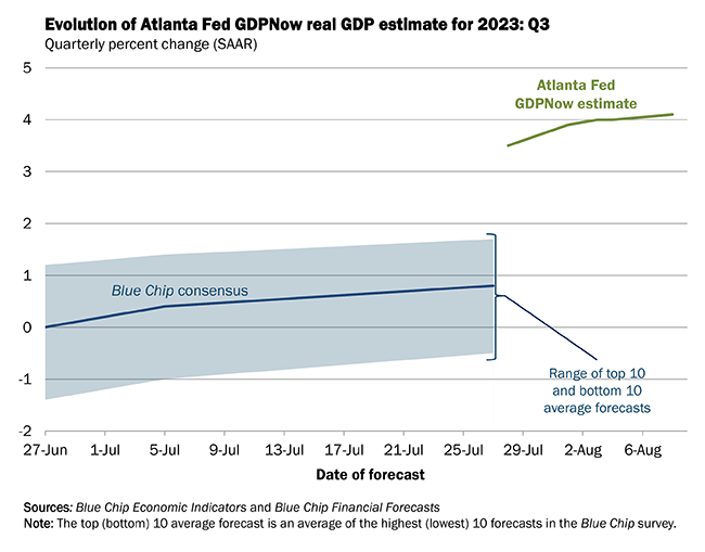
The GDPNow model estimate for real GDP growth (seasonally adjusted annual rate) in the third quarter of 2023 is 4.1 percent on August 8, up from 3.9 percent on August 1. After recent releases from the U.S. Census Bureau, the Institute for Supply Management, the U.S. Bureau of Economic Analysis, and the U.S. Bureau of Labor Statistics, an increase in the nowcast of third-quarter real gross private domestic investment growth from 5.2 percent to 8.1 percent was slightly offset by decreases in the nowcasts of third-quarter real personal consumption expenditures growth and third-quarter real government spending growth from 3.5 percent and 2.9 percent, respectively, to 3.2 percent and 2.7 percent, while the nowcast of the contribution of the change in real net exports to second-quarter real GDP growth increased from 0.08 percentage points to 0.11 percentage points.

The next GDPNow update is Tuesday, August 15.

FRBSF Economic Letter: Can Monetary Policy Tame Rent Inflation?

[from the Federal Reserve Bank of San Francisco Economic Letter]

by Zheng Liu and Mollie Pepper

Rent inflation has surged since early 2021. Because the cost of housing is an important component of total U.S. consumer spending, high rent inflation has contributed to elevated levels of overall inflation. Evidence suggests that, as monetary policy tightening cools housing markets, it can also reduce rent inflation, although this tends to adjust relatively slowly. A policy tightening equivalent to a 1 percentage point increase in the federal funds rate could reduce rent inflation as much as 3.2 percentage points over 2½ years.

“We’ve had a time of red-hot housing market all over the country… Shelter inflation is going to remain high for some time. We’re looking for it to come down, but it’s not exactly clear when that will happen. Hope for the best, plan for the worst.”

Federal Reserve Chair Jerome Powell (2022)

The rapid run-up of shelter costs—both house prices and rents—during the recovery from the pandemic has raised questions about how inflation pressures might affect housing affordability. Since March 2022, the Federal Reserve has rapidly lifted its federal funds rate target from near zero to over 4%, and policymakers have signaled that they are open to keeping the monetary policy stance sufficiently restrictive to return inflation to the longer-run goal of 2% on average. The tightened financial conditions following those policy changes, especially the surge in mortgage interest rates, have helped cool house price growth. However, rent inflation remains elevated.

This Economic Letter examines the effectiveness of monetary policy tightening for reducing rent inflation. We estimate that, during the period from 1988 to 2019, a policy tightening equivalent to a 1 percentage point increase in the federal funds rate can reduce rent inflation—measured by 12-month percentage changes in the personal consumption expenditures (PCE) housing price index—by about 3.2 percentage points, but the full impact takes about 2½ years to materialize. Based on housing costs’ share in total PCE, this translates to a reduction in headline PCE inflation of about 0.5 percentage point over the same time horizon.

Rising housing costs

Following the COVID-19 recession, house prices and rents both surged in the United States. For example, the 12-month growth rate of Standard & Poor’s CoreLogic Case-Shiller Home Price Index accelerated from about 10% in December 2020 to over 20% in March 2022. After the Federal Reserve started raising the target for the federal funds rate in March, house price growth has slowed significantly, to about 9% in October 2022.

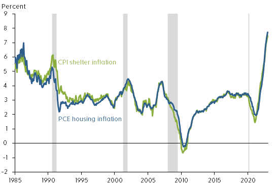
Rent inflation also accelerated during the pandemic period. Figure 1 shows that rent inflation—measured using 12-month changes in the PCE housing price index and including rents for tenant-occupied housing and imputed rents for owner-occupied housing—rose from a low point of about 2% in early 2021 to 7.7% by December 2022, the highest level since 1986. During the same period, rent inflation measured by 12-month changes in the shelter component of the consumer price index (CPI) experienced a similar increase. Thus, following the tightening of monetary policy, house price growth has slowed but rent inflation continues to rise.

Figure 1: PCE and CPI measures of rent inflation
Source: Bureau of Economic Analysis, Bureau of Labor Statistics, and Haver Analytics.
Note: Twelve-month percentage changes. Gray shading indicates NBER recession dates.

Economic theory suggests that some common forces such as changes in housing demand can drive both rents and house prices. For example, the expansion of remote work since the COVID-19 pandemic has increased demand for housing, raising both house prices and rents (Kmetz, Mondragon, and Wieland 2022). To the extent that the stream of current and future rents reflects the fundamental value of a house, house prices can be a leading indicator of future rent inflation (Lansing, Oliveira, and Shapiro 2022). Thus, monetary policy can affect both house prices and rents by cooling housing demand.

Housing demand responds to changes in financial conditions, such as increases in mortgage interest rates. However, theory suggests that house prices are more sensitive than rental prices to changes in financial conditions, because home purchases typically require longer-term mortgage financing. In addition, unlike rents, house prices can be partly driven by investor sentiments or beliefs, which explains the observed larger swings in house prices than in rents over business cycles (Dong et al. 2022). Long-term rental contracts can also contribute to slow adjustments in rent inflation.

Rent inflation is an important contributor to overall inflation because housing costs are an important component of total consumption expenditures. On average, housing expenditures represent about 15% of total PCE and 25% of the services component of PCE. In CPI, shelter costs represent an even larger share, accounting for about 30% of total consumption of all urban consumers and about 40% of core consumption expenditures excluding volatile food and energy components.

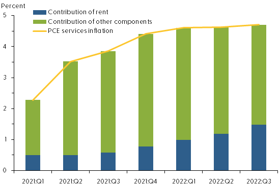
The contribution of rent inflation to overall PCE inflation has increased since early 2021. As Figure 2 shows, in the first quarter of 2021, rent inflation accounted for about 22% of the four-quarter change in the PCE services price index, excluding energy: 0.5 of the 2.3 percentage points increase in service prices was attributable to rent inflation. By the third quarter of 2022, the contribution of rent inflation had climbed to about one-third, or 1.5 of the 4.7 percentage point increase in service prices.

Figure 2: Rising contribution of rent inflation to services inflation
Source: Bureau of Economic Analysis, Haver Analytics, and authors’ calculations.
Note: Four-quarter changes in PCE services price index excluding energy.

Measuring policy effects

Given the rising contribution of rent inflation to overall inflation, it is important to assess the quantitative effects of monetary policy tightening on rent inflation.

For our analysis, we use a measure of monetary policy surprises constructed by Bauer and Swanson (2022). Their measure focuses on high-frequency changes in financial market indicators within a short period surrounding the Federal Open Market Committee (FOMC) policy announcements. If the public fully anticipates a policy change, then the financial market would not react to new policy announcements. However, if the market does react to an announcement, then the policy change must contain a surprise element. Thus, changes in financial market indicators, such as the price of Eurodollar futures, in a narrow window around an FOMC announcement can capture policy surprises. In practice, however, the data constructed this way are not complete surprises because they can be predicted by some macro and financial variables shortly before FOMC announcements. We follow the approach of Bauer and Swanson (2022) to purge the influences of those macro and financial variables from the measure of policy surprises. We use the resulting quarterly time series to measure monetary policy shocks, with a sample period from 1988 to 2019.

We then use a local projections model—a statistical tool proposed by Jordà (2005)—to project how rent inflation responds over time to a tightening of monetary policy equivalent to a 1 percentage point unanticipated increase in the federal funds rate in a given quarter. The model takes into account how monetary policy shocks interact with other macroeconomic variables, including lags of rent inflation, real GDP growth, and core PCE inflation.

In the final step, we compute the responses of rent inflation relative to its preshock level over a period up to 20 quarters after the initial increase in the federal funds rate.

Gradual impact of policy tightening on rent inflation

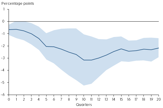
Figure 3 shows the response of rent inflation during the first 20 quarters after an unanticipated tightening of monetary policy (solid blue line). The shaded area shows the confidence band, indicating the statistical uncertainty in estimating the responses. Under the assumption that the model is correct, the shaded area contains the actual value of the rent inflation responses to the monetary policy shock roughly two-thirds of the time. The policy shock is normalized such that it is equivalent to a 1 percentage point unanticipated increase in the federal funds rate.

Figure 3: Response of rent inflation to monetary policy tightening
Source: Bureau of Economic Analysis, Bauer and Swanson (2022), and authors’ calculations.
Note: Response of rent inflation to a monetary policy shock equivalent to a 1 percentage point surprise increase in the federal funds rate. Shaded region shows 68% confidence band around the estimate.

The figure shows that monetary policy tightening has significant and gradual effects on rent inflation. On impact, a 1 percentage point increase in the federal funds rate reduces rent inflation about 0.6 percentage point relative to its preshock level. Over time, rent inflation declines gradually, falling about 3.2 percentage points in the 10 quarters following the impact. The slow adjustment in rent inflation partly reflects the stickiness in nominal rents due to long-term rental contracts. Since housing expenditures account for about 15% of total PCE, this estimate translates to a reduction in headline PCE inflation of about 0.5 percentage point, stemming from the decline in rent inflation over a period of 2½ years.

The rent component of PCE is measured based on average rents, including those locked in long-term rental contracts, which are slow to adjust to changes in economic and financial conditions. Rents on new leases, however, are more flexible. For example, the 12-month growth in Zillow’s observed rent index, which measures changes in asking rents on new leases, has slowed significantly since March 2022 (see Figure 4). Asking rents are typically a leading indicator of future average rents. Thus, the slowdown in asking rent growth could portend lower future rent inflation.

Figure 4: Year-over-year observed rent growth starting to slow
Source: Zillow and Haver Analytics.
Note: Twelve-month percentage changes in Zillow’s observed rent index. Gray shading indicates NBER recession dates.

Conclusion

Rents are an important component of consumer expenditures. Recent surges in rent inflation have led to concerns that overall inflation might stay persistently high despite tightening of monetary policy. We present evidence that monetary policy tightening is effective for reducing rent inflation, although the full impact takes time to materialize. A policy tightening equivalent to a 1 percentage point increase in the federal funds rate can reduce rent inflation up to 3.2 percentage points over the course of 2½ years. This translates to a maximum reduction in headline PCE inflation of about 0.5 percentage point over the same time horizon. Although average rents are slow to respond to policy changes, growth of asking rents on new leases has started to slow following recent monetary policy tightening. Our finding suggests that this tightening will gradually bring rent inflation down over time, thereby helping to reduce overall inflation.

Zheng Liu — Vice President and Director of the Center for Pacific Basin Studies, Economic Research Department, Federal Reserve Bank of San Francisco

Mollie Pepper — Research Associate, Economic Research Department, Federal Reserve Bank of San Francisco

[Archived PDF]

Economy-Watching: U.S. Market Probability Tracker Updated with June’s Employment Data

[from the Federal Reserve Bank of Atlanta]

The following information is now available on the Federal Reserve Bank of Atlanta’s website.

Market Probability Tracker Updated with New Employment Data
On Friday, the U.S. Bureau of Labor Statistics released June’s employment report. Find out how this affected the market’s assessment of future rate moves at the Market Probability Tracker.

U.S. Labor Trends: Atlanta Fed’s Labor Market Tracking Tools Updated with May Data

[from the Federal Reserve Bank of Atlanta’s Center for Human Capital Studies]

What do May employment data from the U.S. Bureau of Labor Statistics mean for the outlook for labor markets? Find out in the Atlanta Fed’s Labor Market Distributions Spider Chart, Jobs Calculator, and Labor Market Sliders.

Want to see even more economic data? Our EconomyNow app will put GDPNow and all our data tools right in your hands. Download it today to see the latest data on inflation, growth, and the labor market.

Essay 48: Bureau of Economic Analysis Materials for Every Student Regardless of Major

We mentioned in a previous essay that an economist receives certain Bureau of Economic Analysis and Bureau of Labor Statistics updates and that allows them to “guesstimate” next year’s GDP growth by adding up average labor productivity growth (Y/L) to labor force growth. Remember Y (GDP) equals Y/L multiplied by L and percentage growth in Y is approximately equal to the sum of the other two variables: Y/L and L.  The sum approximates GDP growth and requires no mental gymnastics with complex mathematics of any kind.  A wise student would learn what’s on offer by these government update services and realize simple familiarity is half the game in everything.  The economics pundits are not ten feet tall.  They simply follow simple materials that the typical student does not have and has no idea that these materials exist.

BEA News:  Gross Domestic Product by Industry, 2nd quarter 2019 and annual update:

“The U.S. Bureau of Economic Analysis (BEA) has issued the following news release today:

“Professional, scientific, and technical services; real estate and rental and leasing; and mining were the leading contributors to the increase in U.S. economic growth in the second quarter of 2019. The private goods‐ and services‐producing industries, as well as the government sector, contributed to the increase.  Overall, 14 of 22 industry groups contributed to the 2.0 percent increase in real GDP in the second quarter.”

The full text of the release [archived PDF] on BEA’s website can be found here

The Bureau of Economic Analysis provides this service to you at no charge.  Visit us on the Web at www.bea.gov.  All you will need is your e-mail address.  If you have questions or need assistance, please e-mail subscribe@bea.gov

Essay 5: How to Sneak Up on a Field With Types of Meta-Intelligence

If you look at a typical economics book and are coming at it with no particular background (e.g., your dad was an economist at the World Bank, say, so you’ve “swum” in this water via your background and dinner table conversations), you will find it “remote” and “foreign.”

What to do? You need to “sneak up” on a field and find a door into it or a window to climb through that brings you inside.

This foreignness and remoteness is true for any field you can think of since unfamiliar fields are disorienting at first. You need a pre-understanding.

Let’s do two simple examples of how one gets a pre-understanding:

During the foreclosure crisis following the Great Recession of 2008 and thereafter, you might have asked yourself about the size in dollars of US residential housing stock to see what it might mean if values declined. You found perhaps that it was surprising difficult to come up with some “ballpark” sense of US housing as you looked through Google and other entries.

Here’s a sample of a kind of made-up workaround that points you in the right direction:

Suppose we say the population of the USA is 320 million at the time, in round figures that are convenient and approximate only.  Assume, for no reason, that all Americans are members of households of four (i.e., families with two parents and two children). This is of course utterly false but serves our “guesstimating” purpose we hope.

If we divide the total population by 4, we get 80 million families. Assume all families live in single-family homes ignoring apartment buildings, multi-family homes and a zillion other forms. Make up a number like 300 thousand dollars per home at the time, based on radio news,  and you will get a national housing stock value of 80 million by 300 thousand which is 24 trillion dollars.

In fact, the official value of U.S. residential housing was usually given at 24-25 trillion so our “sneaking up” guesstimating was not bad at all.

Now ask how one might have perhaps done it better, more cleverly. You have to “back into” a field by something you yourself look into and figure out before you enter the “ocean” of the textbook presentation.

It requires a kind of “sneaking up” on a field with back-of-the-envelope “meta-intelligence” in order for you to attune yourself to the field, or if you want to “parachute” in like a “knowledge spy” and get what you need. This is true for all fields. Some “homemade” familiarity you make up yourself is needed.

How to “Sneak Up” on Academic Fields With Meta-Intelligence

An accepted workhorse of economics is the Cobb-Douglas production function based on two people with the names of Cobb and Douglas.

Your economy produces, say, shirts and to do that you need machines (capital), workers (labor), energy, materials.

Think of 100 women seamstresses at one hundred tables with sewing machines plugged into 100 electrical outlets (energy) and lots of fabric (raw materials for shirt-making).

Capital (e.g., machines, equipment, structures) is denoted by the letter K (from German word Kapital), workers or labor force by L (for labor) and the whole is called KLEM. (capital, labor, energy, materials). The letter A stands for “technology level.”

We simplify and worry only about K and L just to make the math much easier. Remember capital here means machines and not money.

In Cobb-Douglas “world,” the product of your economy, shirts is called Y (we don’t have the shirt prices to keep things easier).

Then Y=A multiplied by K (to the alpha) multiplied by L (to the beta). Alpha and beta are measures of responsiveness, “elasticity,” sensitivity.

Cobb-Douglas is multiplicative (i.e., A by K by L, so the algebra goes easier). A is called “technical change” or technology.

Suppose you don’t know or don’t remember log differentiation (calculus) to easily “play  with” this little equation. That’s ok.

Think of the simple identity z=xy. This could be 10=5 x 2 or 12=4 x 3. You can show that if the left side goes up by 10%, the right must grow by 10 percent so that the 5, say, becomes 5.5. 5.5 x 2 is 11 so both sides are the same again, 11=11. It’s easy to show that the percentage growth on the left side of the equation is roughly the sum of the percentage growth of each of the numbers on the right.

You can easily show that the percentage growth of Y (say 6% per year) is approximately equal to the percentage change of A plus percentage growth of K+ plus that of L with K and L modified by alpha and beta.

This is a simplified version of so-called “Growth accounting” (i.e., components of growth in Y from year to year).

You will find that once you sense how this kind of “accounting” looks and works you can proceed to other kinds of accounting in economics such as Balance of Payments accounting or National Income accounting.

These exercises are key to economics as a field with its textbooks and again you have to sneak into it, so to speak, by climbing through a door or window you made up yourself to give you some bearings.

We call all this a pre-understanding before more usual understanding through textbooks.

Pre-understanding is a deep key or prerequisite to educational mastery.

On a National Public Radio call-in talk show few years ago, there was a discussion by four economists (professors plus private sector analysts). A listener calls in and asks one of them about the growth prospect for the following year. The professor responds: about 2.88 percent. Everybody goes quiet and wonder how he figures this out.

The answer will help you “sneak in” to or “parachute” into this world.

The professor, in his mind, calls the economy Y. He realizes that Y is the same as Y/L multiplied by L, where L is labor force. In Y/L by L the l’s cancel each other out so it’s just a harmless re-write of the basic variable Y.

Y/L is average productivity (e.g., number of shirts [the economy has one product, shirts]) divided by number of workers (laborers, seamstresses making the shirts).

If Y is one hundred and L=10, then the average laborer produced 100/10=10 shirts. ie that’s the average productivity.

The professor knows that approximately the percentage growth of Y (which is what the radio show caller’s question was about) is the sum of the percentage growth of Y/L and L.

He’s familiar with the latest productivity and labor force projections from the electronic newsletters he receives and the websites he checks out (e.g., BEA and the BLS, et al).

He adds them up to get 2.88 percent, the number he mentions to the questioner and the rest of the radio audience.

Once you’re familiar with these simple elements of analysis and sources of info, you can begin to lose your fearfulness and do the same as the professor, who is not solving complex differential equations in his head to answer the question for the listeners.

As a “field outsider,” you’re unfamiliar with the “landscape” and “rules of thumb” and your mind races or wanders when confronted by such a question because you don’t have these simple techniques.

You can thus “parachute” into any field and leave with what you need.